Signal-analysis background
The cleanest way to see why the pulse below excites many spectral components is to start from the continuous Fourier transform. For a time-dependent signal $h(t)$, define
\[\hat h(\omega) = \int_{-\infty}^{\infty} h(t)e^{-i\omega t}\,dt, \qquad h(t) = \frac{1}{2\pi} \int_{-\infty}^{\infty} \hat h(\omega)e^{i\omega t}\,d\omega.\]This pair of formulas says that a time signal can be decomposed into monochromatic components $e^{i\omega t}$. A perfectly monochromatic component has one exact frequency, but it extends over all time. A finite pulse is the opposite kind of object: it is localized in time, so its Fourier transform must occupy a finite frequency band.
For example, if a carrier is multiplied by a temporal envelope,
\[h(t)=g(t)\cos(\omega_0 t+\varphi_0),\]then the spectrum is centered near $\pm\omega_0$, but its width is controlled by the envelope $g(t)$. Shortening $g(t)$ broadens $\hat h(\omega)$. This is the first version of the tradeoff that will later reappear in the cavity-mode projection.
In numerical work this tradeoff appears in an even more concrete form. Suppose the signal is sampled with time step $\Delta t$ and $N$ samples. The total time window is
\[T=N\Delta t.\]The Fourier frequencies are separated by
\[\Delta f=\frac{1}{T}, \qquad \Delta\omega=\frac{2\pi}{T}.\]Thus the frequency resolution is controlled by the total time range: a longer time record gives a finer frequency grid. The largest resolvable frequency is controlled by the sampling interval:
\[f_{\max}\simeq \frac{1}{2\Delta t}, \qquad \omega_{\max}\simeq \frac{\pi}{\Delta t}.\]In this sense the bookkeeping is:
- time resolution: $\Delta t$,
- time range: $T=N\Delta t$,
- frequency resolution: $\Delta f=1/T$, or $\Delta\omega=2\pi/T$,
- frequency range: set by the sampling rate, up to the Nyquist scale $1/(2\Delta t)$.
Nothing in this reasoning is special to time. If a spatial field $u(x)$ is expanded as
\[\tilde u(k) = \int_{-\infty}^{\infty} u(x)e^{-ikx}\,dx, \qquad u(x) = \frac{1}{2\pi} \int_{-\infty}^{\infty} \tilde u(k)e^{ikx}\,dk,\]then $k$ plays the same role for space that $\omega$ plays for time. For a spatial grid with spacing $\Delta x$ over a length $L=N\Delta x$,
\[\Delta k=\frac{2\pi}{L}, \qquad k_{\max}\simeq \frac{\pi}{\Delta x}.\]Increasing the real-space window improves $k$-space resolution. Refining the real-space grid extends the available $k$-space range. Conversely, making a source local in $x$ necessarily spreads it in $k$.
The continuous statement behind these tradeoffs is the time-frequency uncertainty relation. If $\Delta t$ and $\Delta\omega$ are measured as standard deviations of the signal and its Fourier transform, then
\[\Delta t\,\Delta\omega\geq \frac{1}{2}.\]The spatial analogue is
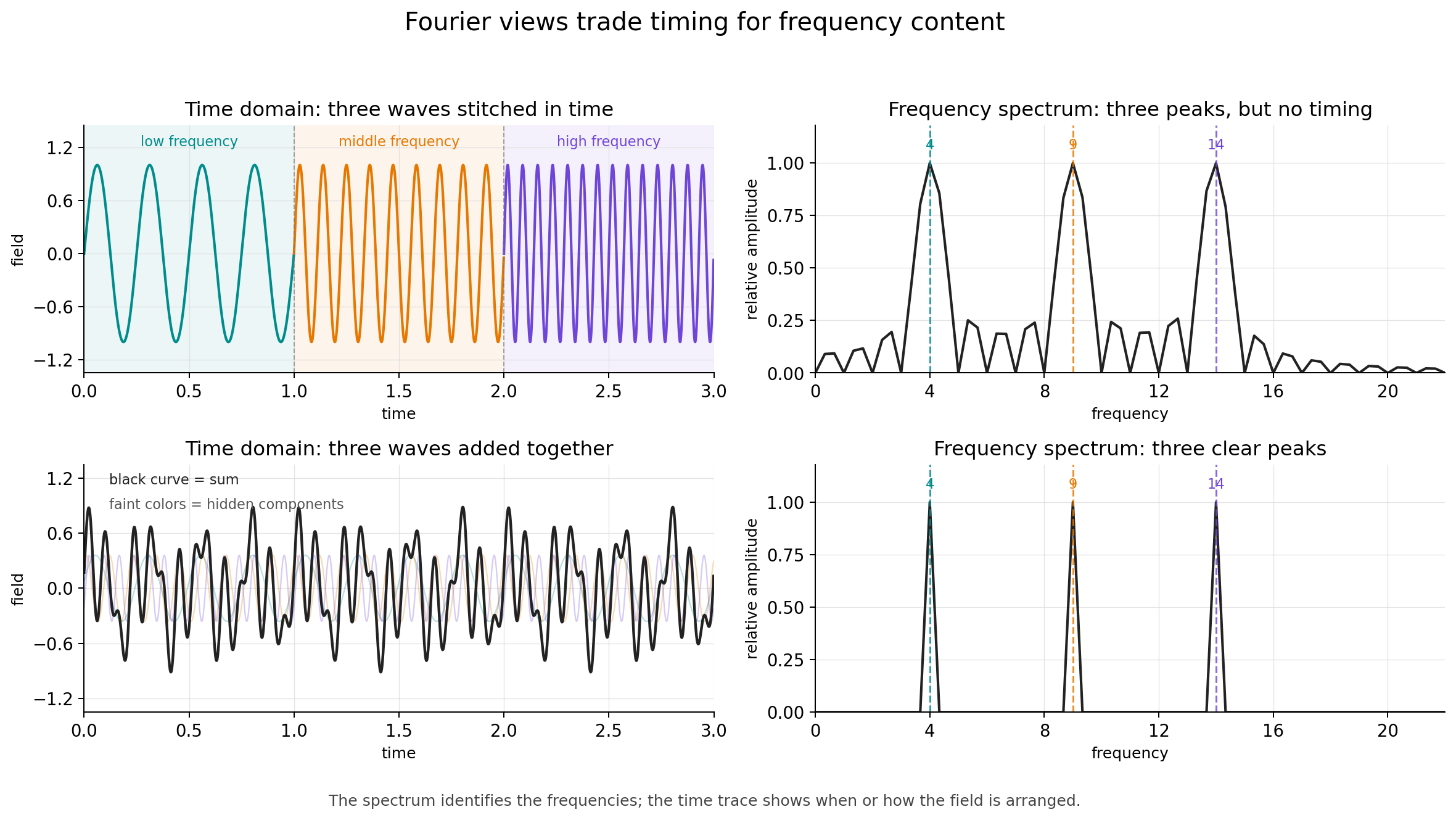
\[\Delta x\,\Delta k\geq \frac{1}{2}.\]This means that the two descriptions cannot both be made arbitrarily sharp at the same time. A signal that is very localized in time must occupy a broad frequency band, and a source that is very localized in position must occupy a broad range of wavevectors. The Fourier transform connects these paired descriptions, but each representation hides something that the other makes explicit: a time trace shows when the field is present without directly labeling its frequency content, while a frequency spectrum shows which components are present without saying when they appeared.
As a concrete example, imagine stitching together three different plane waves over three separate time intervals. The Fourier spectrum would show three peaks, but the peaks alone would not reveal the order or timing of the three waves. Conversely, if three plane waves are present at the same time, their superposition may look complicated enough that the number of underlying components is not obvious from the time-domain curve alone.
One way to keep both pieces of information visible is to stop using infinitely extended plane waves as the only analysis basis. The Fourier transform expands a signal in the basis $e^{i\omega t}$, whose frequency is perfectly sharp but whose time location is completely delocalized. Wavelet analysis replaces this by translated and rescaled localized oscillations. A common choice is a Gaussian packet multiplied by a plane wave,
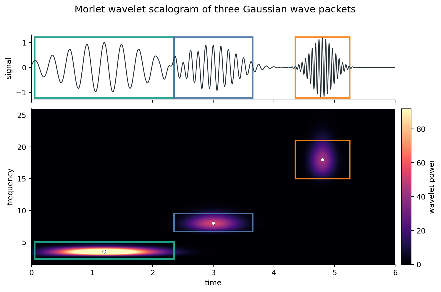
\[\psi_{t_0,\omega_0}(t) = \exp\left[ -\frac{(t-t_0)^2}{2\sigma_t^2} \right] e^{i\omega_0(t-t_0)}.\]This object is called a Morlet wavelet, or Gabor wavelet depending on convention and normalization. It is not infinitely sharp in either time or frequency, but it has a controlled width in both. Sliding it along the signal and changing its central frequency gives a time-frequency map: bright regions mark where the signal locally resembles that wavelet.
For example, the following synthetic signal contains three Gaussian wave packets placed at roughly equal time intervals. The first packet has a low carrier frequency and a long envelope, the second has an intermediate frequency and duration, and the third has a high carrier frequency and a short envelope. The wavelet scalogram reflects the useful side of the time-frequency tradeoff: at low frequency, the signal lasts long enough that precise timing is less important, so the map gives a narrow frequency band spread over a longer time interval; at high frequency, the signal is brief, so the map sacrifices some frequency sharpness while clearly locating when the packet appears.
Wavelet pulse in MaxwellLink
The k_parallel_pulse in MaxwellLink has the schematic real-space form
where $W(x)$ is the finite spatial source window. In the examples considered here, $g(t)$ is a Gaussian pulse envelope with adjustable center and width, for example
\[g(t) = \exp\left[ -\frac{(t-t_c)^2}{2\sigma_t^2} \right],\]where $t_c$ sets the pulse center and $\sigma_t$ sets its temporal width. Multiplying the carrier by this envelope makes the drive strongest near $t_c$ and suppresses it away from that time. A smaller $\sigma_t$ gives a shorter pulse, while a larger $\sigma_t$ gives a longer, more nearly monochromatic drive.
The carrier $\omega_0$ sets the central frequency, and $k_\parallel$ sets the intended central in-plane wavevector. However, the actual excitation is not a delta function at exactly $(\omega_0,k_\parallel)$. A delta-like frequency component would require an infinitely long monochromatic signal, while a delta-like wavevector component would require an infinitely extended spatial source. Here both the temporal envelope and the spatial source window are finite.
For this Gaussian convention, the Fourier transform of $g(t)$ is also Gaussian:
\[\hat g(\omega) \propto \sigma_t \exp\left[ -\frac{\sigma_t^2\omega^2}{2} \right] e^{-i\omega t_c}.\]Thus, if the temporal width is measured by the standard deviation of the amplitude envelope, then the angular-frequency width is
\[\sigma_\omega=\frac{1}{\sigma_t},\]so the product is $\sigma_t\sigma_\omega=1$. If one instead measures the intensity width, or quotes a full width at half maximum, the numerical prefactor changes, but the scaling remains $\Delta\omega\propto 1/\sigma_t$.
If the source window has an effective length $L_{\mathrm{src}}$ along the propagation direction, then its wavevector width is on the order of
\[\Delta k \sim \frac{1}{L_{\mathrm{src}}}.\]The common real-space source
Let the molecular grid points be $\mathbf r_i=(x_i,y_i)$, where $x_i$ and $y_i$ are fractional cavity coordinates. Let the source be centered at $\mathbf r_0=(x_0,y_0)$. We first selects grid points inside a rectangular source region. If the full source size is $(L_x^{\mathrm{src}},L_y^{\mathrm{src}})$, then point $i$ is selected when
\[|x_i-x_0|\leq \frac{L_x^{\mathrm{src}}}{2}, \qquad |y_i-y_0|\leq \frac{L_y^{\mathrm{src}}}{2}.\]Inside that region, MaxwellLink applies a smooth Hann window. Denote it by $W_i$.
For direction="x" the spatial phase is
For direction="y", it is
For a two-dimensional in-plane direction, the phase is
\[\phi_i = \pi\frac{k_{\parallel,x}}{\Delta\omega_x}(x_i-x_0) + \pi\frac{k_{\parallel,y}}{\Delta\omega_y}(y_i-y_0).\]Thus the intended local carrier has the form
\[\cos(\omega t-\phi_i+\varphi_0),\]multiplied by a temporal envelope $g(t)$, the spatial window $W_i$, and an amplitude $A$.
Route 1: target="molecule"
When target="molecule", the returned function _drive(t) produces one scalar value for each selected molecular grid point as the external pulse:
Therefore the shape of _drive(t) is $(\mathrm{len}(\texttt{source.excited_grid_list}),)$. In the multimode solver, this pulse is added directly to the effective electric field seen by the selected molecular drivers:
Here $\hat{\mathbf e}_{\mathrm{mol}}$ is chosen by molecule_pulse_axis, for example "y". In code, this happens in _step_molecules, where _eval_pulse_field broadcasts a scalar array of shape $(\mathrm{len}(\texttt{source.excited_grid_list}),)$ into a vector-valued array of shape $(\mathrm{len}(\texttt{source.excited_grid_list}),3)$.
Route 2: target="photon"
When target="photon", MaxwellLink does something different. It uses the same source window and phase, but projects the complex spatial source onto cavity mode functions. Let the selected polarization component be $\alpha$, controlled by projection_axis. The mode projection is
The code then normalizes these coefficients by their largest magnitude:
\[\tilde c_k = \frac{c_k}{\max_j \lvert c_j\rvert}.\]Only modes satisfying
\[\lvert c_k\rvert > 10^{-12}\max_j \lvert c_j\rvert\]are kept in source.excited_mode_list. The returned _drive(t) is then
Thus, for photonic targeting, the shape of _drive(t) is equal to whole photon mode $(n_{\rm mode},)$.
Why a local photon pulse often excites many modes
Consider the common one-dimensional case with
y_grid_1d = [0.0]
coupling_axis = "y"
projection_axis = "y"
For the Fabry-Perot mode functions used in FabryPerotCavity, the $y$-polarized component is
The photonic projection is therefore approximately
\[c_\ell = \sum_{i\in\mathrm{src}} 2\sin(\ell\pi x_i) W_i e^{-i\phi_i}.\]A finite-width wavepacket is not a single sine mode. It has a broad spectrum in the cavity basis. Unless symmetry makes a coefficient exactly vanish, most $c_\ell$ are nonzero. Since the code keeps all modes above a relative threshold of $10^{-12}$, a localized photonic source can easily excite every available mode in the truncated basis.
This does not mean every mode is excited equally. The amplitudes are encoded in $\tilde c_k$. It only means that the returned vector includes all modes whose projection is numerically nonzero.
Why the two routes need not look identical
Although target="photon" is built from the same real-space source pattern, it is not just the molecular pulse written in another variable. Several additional operations intervene:
- projection onto the cavity mode basis,
- truncation to the available finite set of modes,
- normalization by $\max_k \lvert c_k\rvert$,
- selection of a polarization component through
projection_axis, - propagation through the driven oscillator equation for $q_k$,
- reconstruction of the real-space field from the mode coordinates.
Consequently, a molecular excitation and a photonic excitation can differ in apparent launch position, phase, or wavepacket slope if the projection basis, signs, normalization, or pulse axes are not carefully matched.
There is also a practical sign convention to watch. The effective electric field from the cavity coordinate is computed with
\[\mathbf E_k(\mathbf r,t) = -\varepsilon_k q_k(t)\mathbf f_k(\mathbf r).\]Thus a positive drive on $q_k$ does not necessarily correspond to a positive local electric field at the molecule. When comparing a direct molecular field pulse to a mode-coordinate drive, this extra sign convention must be kept in mind.